I said before that I don’t want to get into the details of how LemonGraph is dealing with parsing the queries. Unfortunately, I can’t avoid that. There seems to be a lot of logic, magic and mystery in the MatchLGQL() class, which is critical to understanding how queries work.

The problem is that either my Python-fu is lacking or it is just really hard to figure out a non trivial codebase behavior in a dynamic language like python. I find it hard to figure out what data is stored where and how it is manipulated. Therefor, I decided to break with my usual custom and actually run the code in the debugger to try to follow what is going on there. I tried to run this on WSL, but it crashed horribly, so I had to spin up a VM and setup PyCharm on it. First time that I’m actually using that and the experience is pretty nice so far. Being able to inspect things directly means that it is much easier to figure out the behavior of the code.

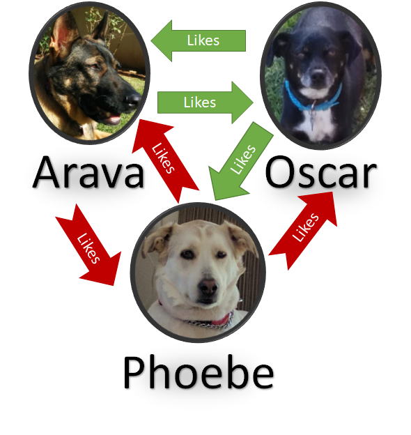
In order to explore how queries work in LemonGraph, I created the following graph, which represents the relationships between my dogs:

Here is how this looks like in code:

This tells us to find all the dogs that like each other. And it finds:

• Arava –> Oscar
• Oscar –> Arava
• Oscar –> Pheobe

Now that we have a query that we can sink our teeth into, let’s figure out how this work, shall we? Inside the dreaded MatchLGQL() class, there are all sorts of regular expressions running on the parse this thing, but eventually we get to the partially processed parsed query:

This screen shot might explain why I wasn’t happy with the code structure for figuring out what is going on without debugging. The number of tuples here is quite amazing, and they are used everywhere. This make static analysis (as in, just reading the code) too hard for me. But with the debugger, that is much easier. If you are familiar with ASTs, this should be pretty easy to figure out.

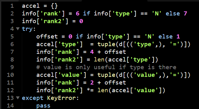
Here is a piece of code that we already looked at (and criticized), this is in munge_obj() method, where it is deciding how to optimize the query:

This piece of code is critical for the performance of the system. And it is really hard to understand. Here is what is going on.

The accel array tell a later piece of code how to accelerate the query, using the type or type and value to start from a particular source. The info is used to carry state about particular clause in the query. Before this code run there is some code that builds the dictionary d which is used to figure out the filters on the particular clause. This is fun, because it is using missing a key lookup in the dictionary for control flow.

Let’s follow the logic?

• Line 2 - If the clause operates on a node, rank it as 6. If it is an edge, rank it as 7.
• Line 6 – If the clause has a type specified, rank is as 4 if it is a node, 5 if it is an edge. Otherwise, abort the optimization.
• You might not see the “abort this optimization” in line 6, because it relies on the dictionary to throw if the key isn’t found. This is a common pattern in this code and something that I personally greatly dislike.
• Line 8 – it uses the length of the type as a metric for secondary ranking. I’m not quite sure why this is the case. I guess the code needed a tie breaker, but I can’t imagine why the length of a type would have any impact on performance.
• Unless, of course, the code assumes that shorter types are more common, and therefor will prefer to use the rare longer types?
• Line 10 – If there is a type and a value defined, that is even better. Note that again the is the ranking of node (2) and edge (3) which I find non obvious.

Here are the results of the matches after they have been munged, I marked the ranking:

Looking at this, this seems very strange, the rank2 value is 1 in the second element, but I expected it to be the length of the string. As it turns out, this is not working directly on the string, it is working on the tuple of possible values, so the secondary ranking here is not based on the length of the type or the value but on the number of possible types and values that were specified for each clause.

The code judges that the best place to start this query is with the second entry, since it is the most specific option. This in turn takes us the the seeds() method that we previously covered. In this case, the code is going to hit this branch:

This means that it is going to be iterating over all the edges of a particular type and filtering them in Python code. This is strange, because the on disk indexes actually support doing a direct query on the (type, value) directly and would probably be much cheaper in the case you have many values for a particular type of an edge.

In fact, just that is implemented for querying nodes by (type, value):

I’m guessing that they are either don’t have a lot of queries on (type, value) on edges or not a lot of different values for edge types that they can optimize in this manner.

That is enough for now, I have a pretty good grasp of how queries are parsed and how they fetch data from the underlying storage. The next post will talk about how LemonGraph takes the seeds of the query and execute the actual graph operations on them. The code that does this is tight and will require a full post to explore properly.