Oren Eini

CEO of RavenDB

a NoSQL Open Source Document Database

Get in touch with me:

oren@ravendb.net +972 52-548-6969

Posts: 7,546
|
Comments: 51,161
Privacy Policy · Terms
filter by tags archive
time to read 2 min | 257 words

imageFor my needs, I’m mostly interesting in being able to under this type of query:

from Users
where City = ‘London’
order by LastLogin

I already looked at a few of these, as you can see in past posts. However, as I was trawling through the internet (or, more precisely, though various GitHub projects) I found quite a few search libraries that don’t have ordering support.

For example:

Why would anyone build such a system? Isn’t order by important?

Well, yes and no. In practice, all the libraries I found that skip explicit order by do that for a few good reasons. First, they are focused on IR (information retrieval) rather than queries. In other words, they all absolutely do ordering, but they do that based on how closely they were able to match the results to your query. For such a system, sorting by a different field is not meaningful. You want to have the most relevant results.

The other reason is that ordering by a arbitrary field, unrelated to the query, is tough. You have to explicitly keep track of additional information to be able to do that. IR is already complex enough, and in many cases, what you are searching on is a huge corpus of unstructured (at best, semi structured) data. You can’t afford the cost of tracking more data or the time to try to sort potentially many millions of results.

time to read 2 min | 285 words

In the previous post, I looked into the Bleve search engine library. Now, I want to go into the codebase and answer a simple question. How does Bleve handles sorting of queries. Here is my code:

During the search process, we have visitor defined:

This is called on every field (and term value) that is found in the query (it looks like only the relevant ones are touched, but that is still a lot). Eventually, this gets here:

At this point, we can see that we basically gather a list of of all the terms in the values field inside the UpdateVisitor. This is important, because we are later going to rely on the same order of iteration, as you can see in the Value call. Even though there is a DocumentMatch being passed there, it isn’t actually being used. Instead, it always take the first element in the values.

This is called on a per document level, so there is an expectation that the values will be smaller. On the other hand, during the sorting process, we’ll merge it all into a single location per document, as you can see:

In other words, the doc.Sort is going to end up with an array of the values that we want to sort by. At this point, sorting is done by maintaining a heap and pushing values to it until we get the top N elements. Pretty simple overall.

It also allocates quite heavily, with arrays, slices and strings. I don’t have a good feeling for where it actually will be a problem in Go, but it is something to consider. In C#, I would be very worried about the eventual costs of all of these allocations.

time to read 6 min | 1191 words

Bleve is a Go search engine library, and that means that it hit a few good points with me. It is interesting, it is familiar ground and it is in a language that I’m not too familiar with, so that is a great chance to learn some more.

I reviewed revision: 298302a511a184dbab2c401e2005c1ce9589a001

I like to start with reading from the bottom up, and in this case, the very first thing that I looked at was the storage level. Bleve uses a pluggable storage engine and currently has support for:

  • BoltDB
  • LevelDB
  • Moss
  • In memory tree

This is interesting, if only because I put BoltDB and Moss on my queue of projects to read.

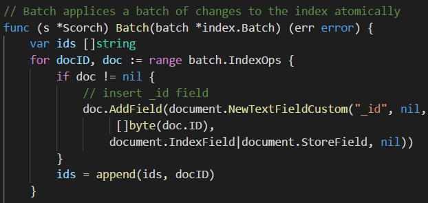
The actual persistent format for Bleve is very well document here. Which make it much easier to understand what is going on. The way Bleve uses the storage, it has a flat key/value store view of the world, as well as needing prefix range queries. Nothing else is required. Navigating the code is a bit hard for me as someone who isn’t too familiar with Go, but the interesting things start here, in scorch.go (no idea why this is called scorch, though).
image

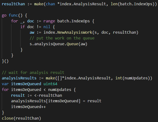
We get a batch of changes, and run over them, adding an _id field to the document. So far, pretty simple to figure out. The next part is interesting:
image

You can see that we are running in parallel here, starting the analysis work and queuing it all up. Bleve then wait for the analysis to run. I’ll dig a bit deeper into how that work in a bit, first I want to understand how the whole batch concept work.
image

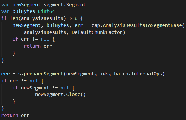
So that tells us some interesting things. First, even though there is the concept of a store, there is also this idea of a segment. I’m familiar with this from Lucene, but there it is tied very closely to the on disk format. Before looking at the analysis, let’s look at this concept of segments.

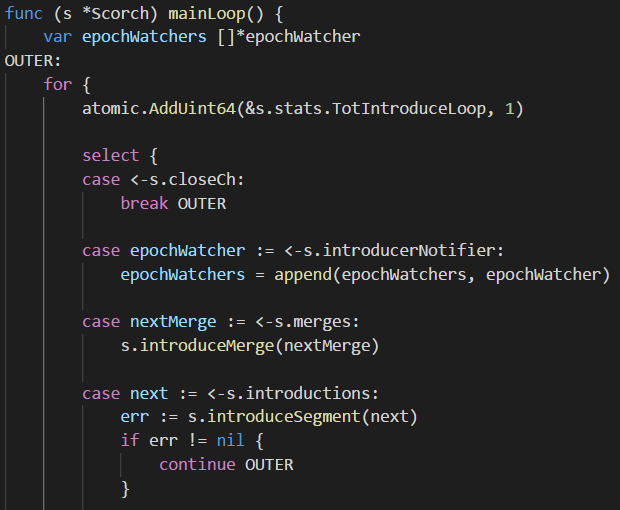
The “zap” package, in this term, seems to refer to the encoding that is used to store the analysis results. It looks like it is running over all the results of the batch and write them into a single binary value. This is very similar to the way Lucene works so far, although I’m still confused about the key/value store. What is happening is that after the segment is created, it is sent to prepareSegment. This eventually send it to a Go channel that is used in the Scortch.mainLoop function (which is being run as a separate thread).

Here is the relevant code:
image

The last bit is the one that is handling the segment introduction, whatever that is. Note that this seems to be strongly related to the store, so hopefully we’ll see why this is showing up here. What seems to be going on here is that there is a lot of concurrency in the process, the code spawns multiple go funcs to do work. The mainLoop is just one of them. The persisterLoop is another as well as the mergerLoop. All of which sounds very much like how Lucene works.

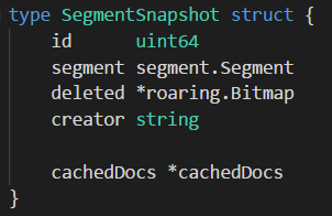
I’m still not sure how this is all tied together. So I’m going to follow just this path for now and see what is going on with these segments. A lot of the work seems to be around managing this structure:
image

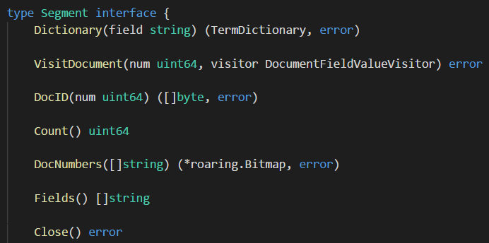
The Segment itself is an interface with the following definition:
image

There are go in memory and mmap versions of this interface, it seems. So far, I’m not following relation between the storage interface and this segments idea. I think that I’m lost here so I’m going to go a slightly different route. Instead of seeing how Bleve write stuff, let’s focus on how it reads. I’ll try to follow the path of a query. This path of inquiry leads me to this guy:

image

Again, very similar to Lucene. And the TermFieldReader is where we are probably going to get the matches for this particular term (field, value). Let’s dig into that. And indeed, following the code for this method leads to the inverted index, called upside_down in this code. I managed to find how the terms are being read, and it makes perfect sense, exactly as expected, it does a range query and parses both key and values for the relevant values. Still not seeing why there is the need for segments.

And here is where things start to come together. Bleve uses the key/value interface to store some data that it searches on, but document values are stored in segments, and are loaded directly from there on demand. At a glace, it looks like the zap encoding is used to store values in chunks. It looks like I didn’t paid attention before, but the zap format is actually documented and it is very helpful. Basically, all the per document (vs. per term / field) data is located there, as well as a few other things.

I think that this is were I’ll stop. The codebase is interesting, but I now know enough to have a feeling how things work. Some closing thoughts:

  • Really good docs.
  • I didn’t use my usual “read the project in lexical file order” to figure out things, and I had a hard time navigating the codebase because of that. Probably my lack of Go chops.
  • There seems to be a lot more concurrency for stuff that I would usually assume be single threaded than I’m used to. I’m aware that Go has builtin concurrency primitives and it is more common to use there, but it seems strange to see. As consume of search libraries, I’m not sure that I’m happy about this. I like to control my threading behaviors.
  • It seems that a lot of the data is held in memory (mmap) but in a format that requires work to handle or in the key/value store, but again, in a format that require work.

The problem with work is that you have to do it each and every time. I’m used to Lucene (read it once from disk and keep a cached version in memory that is very fast) or Voron, in which the data is held in memory and can be access with zero work.

I didn’t get to any of the core parts of the library (analysis, full text search). This is because they aren’t likely to be that different and they are full of the storage interaction details that I just went over.

time to read 3 min | 472 words

After looking at Lucene, the next library that I looked at is the Noise search project. This is a Rust library that is sitting on top of RocksDB. It has a very different model internally than Lucene. You can read a full review I made for this project a while ago.

At any rate, what we are looking at here is this code:

The question here is how are we going to be sorting these results. Digging into the code, ordering is a bit complex to figure out, but I think I got it. The way Noise work, it writes the following values to RocksDB:

  • W.City!Austin#2
  • W.City!Dallas#1
  • W.City!New York#3
  • W.State!NY#3
  • W.State!TX#1
  • W.State!TX#2

These are the values of the relevant documents. I’m ignoring the filtering part of the query, because that isn’t relevant to what I’m trying to find.

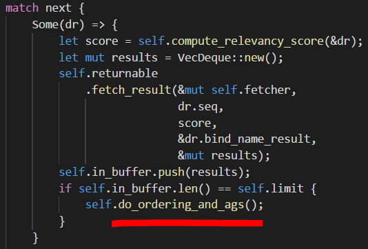
This piece of code is what actually handles the ordering during query retrieval.

image

Notice that this is done in a buffered manner, which is interesting. Let’s go and look at the actual do_ordering_and_ags method. This is a pretty large method, and the relevant piece has about 75 lines of pretty complex logic around how to keep the top N results based on the ordering of the query.

The key part there is that comparing any two results in done using the following code:

image

This ends up being here:

And this is the really interesting piece. The a and b variables are basically each the returned results for each matched document, with the n here being the position of a particular field in the vector.

This has interesting implications. To start with, it means that whenever we have sorting, we have to fetch, in addition to the values we want to return, the values that we want to search by. If there are a lot of results to go through, that can cause a lot of individual queries to RocksDB. It also means that you need to materialize all of that memory directly. The cost of doing comparisons is also non trivial. Noise will actually compare the values directly, so it is expected that the comparison costs will dominate here, especially if you have large values.

Lucene, in the same situation, is able to use the ordinal position and spare a lot of that cost. Noise doesn’t seem to benefit from repeated queries, in each case, the value for each of the sorted field would have to be fetch, compared and sorted individually. On the other hand, the cost if directly proportional to the number of results in the query, vs. the number of documents in the index (for the first query), as it is on Lucene.

time to read 3 min | 537 words

In this series of posts, I am going to take a look at a single feature across several search engine libraries. Given three documents, sort them by State and then by City. This is a pretty trivial query, but there is a lot that is going on behind the scenes that needs to happen for this to actually work. Let’s look at how this is implemented, shall we?

The first library to look at it Lucene, because it is so prevalent. Here is the relevant code that I’m executing:

A key part of the way Lucene executes sorting is this piece of code:

image

As you can see, we ask the reader (a single file in a Lucene directory) to get a the list of field values and matches for a particular field.

In this case, what his means it that doc #0 has the value in lookup[2], doc #1 as well, and doc #2 has the value in lookup[1]. This means that when we compare, we can do it using the following code:

image


And this is called for each field independently, like so:

image

All of which is pretty simple and straightforward. There is a nice optimization here in the sense that in most cases, if the readerGen is the same, we can compare the ordinals directly, without comparing the actual string values.

The problem here is that we need to hold arrays. In particular, I’m talking about the FieldCache.GetStringIndex() (and it’s related friends). The way Lucene stores the values on disk means that on first read, it needs to reconstruct the terms from the index. Here is the core of the work that is done in GetStringIndex.

As you can see, this rips through the entire file, reading each term and then getting all the documents for a particular term. The code is quite clever, because we don’t need to compare anything, we know that we are sorted, so we can take advantage of that when detecting the ordinals.

What this code isn’t very helpful about, though, is the fact that this is allocating a lot of memory. In particular, it will allocate arrays with a value per each document in the index. On large indexes, these can be very large. The good thing here is that there is a good caching going on here, so you’ll typically not need to run this code all too often. The bad thing is that this runs per segment. If you have a lot of small index batches, you’ll have a lot of values like that floating around, and then it will get merged, and you’ll have to run through this again. This is also one of the primary reasons Lucene is limited to about 2.1 billion documents per index.

The good thing about it is that this is really flexible and give us a great performance when sorting.

So now that we know how Lucene does it, let’s look at other libraries.

time to read 4 min | 754 words

RavenDB uses a consensus protocol to manage much of its distributed state. The consensus is used to ensure consistency in a distributed system and it is open for users as well. You can use this feature to enable some interesting scenarios.

The idea is that you can piggy back on RavenDB’s existing consensus engine to gain the ability allow you to create robust and consistent distributed operations. RavenDB exposes these operations using  a pretty simple interface: compare-exchange.

At the most basic level, you have a key/value interface that you can make distributed atomic operations on, knowing that they are completely consistent. This is great, in abstract, but it s a bit hard to grasp without a concrete example.

Consider the following scenario. We have a bunch of support engineers, ready and willing to take on any support call that come. At the same time, an engineer can only a certain number of support calls. In order to handle this, we allow engineers to register when they are available to take a new support call. How would we handle this in RavenDB? Assuming that we wanted absolute consistency? An engineer may never be assigned too much work and work may never be lost. Assume that we need this to be robust in the face of network and node failure.

Here is how an engineer can register to the pool of available engineers.


The code above is very similar to how you would write multi-threaded code. You first get the value, then attempt to do an atomic operation to swap the old value with the new one. If we are successful, the operation is done. If not, then
we retry. Concurrent calls to RegisterEngineerAvailability will race each other. One of them will succeed and the others will have to retry.

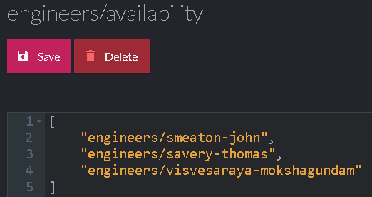
The actual data that we store in the compare exchange value in this case is an array. You can see an example of how that would look here:

img18


Compare exchange values can be simple values (numbers, strings), arrays or even objects. Any value that can be represented as JSON is valid there. However, the only operation that is allowed on a compare exchange value is a wholesale replacement.

The code above is only doing half of the job. We still need to be able to get an engineer to help us handle a support call. The code to complete this task is shown below:


The code for pulling an engineer from the pool is a bit more complex. Here we read the available engineers from the server. If there are none, we'll wait a bit and try again. If there are available engineers we'll remove the first one and then try to update the value. This can happen for multiple clients at the same time, so we check whatever our update was successful and only return the engineer if our change was accepted.

Note that in this case we use two different modes to update the value. If there are still more engineers in the available  pool, we'll just remove our engineer and update the value. But if our engineer is the last one, we'll delete the value
entirely. In either case, this is an atomic operation that will first check the index of the pre-existing value before performing the write.

It is important to note that when using compare exchange values, you'll typically not act on read. In other words, in PullAvailableEngineer, even if we have an available engineer, we'll not use that knowledge until we successfully wrote the new value.
The whole idea with compare exchange values is that they give you atomic operation primitive in the cluster. So a typical usage of them is always to try to do something on write until it is accepted, and only then use whatever value you read.

The acceptance of the write indicates the success of your operation and the ability to rely on whatever values you read. However, it is important to note that compare exchange operations are atomic and independent. That means an operation
that modify a compare exchange value and then do something else needs to take into account that these would run in separate transactions.

For example, if a client pull an engineer from the available pool but doesn't provide any work (maybe because the client crashed) the engineer will not magically return to the pool. In such cases, the idle engineer should periodically check
that the pool still the username and add it back if it is missing.

time to read 4 min | 685 words

I have talked before about RavenDB’s MapReduce indexes and their ability to output results to a collection as well as RavenDb’s ETL processes and how we can use them to push some data to another database (a RavenDB database or a relational one).

Bringing these two features together can be surprisingly useful when you start talking about global distributed processing. A concrete example might make this easier to understand.

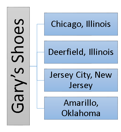
Imagine a shoe store (we’ll go with Gary’s Shoes) that needs to track sales across a large number of locations. Because sales must be processed regardless of the connection status, each store hosts a RavenDB server to record its sales. Here is the geographic distribution of the stores:

img06

To properly manage this chain of stores, we need to be able to look at data across all stores. One way of doing this is to set up external replication from each store location to a central server. This way, all the data is aggregated into a single location. In most cases, this would be the natural thing to do. In fact, you would probably want two-way replication of most of the data so you could figure out if a given store has a specific shoe in stock by just looking at the local copy of its inventory. But for the purpose of this discussion, we’ll assume that there are enough shoe sales that we don’t actually want to have all the sales replicated.

We just want some aggregated data. But we want this data aggregated across all stores, not just at one individual store. Here’s how we can handle this: we’ll define an index that would aggregate the sales across the dimensions that we care about (model, date, demographic, etc.). This index can answer the kind of queries we want, but it is defined on the database for each store so it can only provide information about local sales, not what happens across all the stores. Let’s fix that. We’ll change the index to have an output collection. This will cause it to write all its output as documents to a dedicated collection.

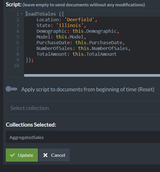
Why does this matter? These documents will be written to solely by the index, but given that they are documents, they obey all the usual rules and can be acted upon like any other document. In particular, this means that we can apply an ETL process to them. Here is what this ETL script would look like.

img07

The script sends the aggregated sales (the collection generated by the MapReduce index) to a central server. Note that we also added some static fields that will be helpful on the remote server so as to be able to tell which store each aggregated sale came from. At the central server, you can work with these aggregated sales documents to each store’s details, or you can aggregate them again to see the state across the entire chain.

The nice things about this approach are the combination of features and their end result. At the local level, you have independent servers that can work seamlessly with an unreliable network. They also give store managers a good overview of their local states and what is going on inside their own stores.

At the same time, across the entire chain, we have ETL processes that will update the central server with details about sales statuses on an ongoing basis. If there is a network failure, there will be no interruption in service (except that the sales details for a particular store will obviously not be up to date). When the network issue is resolved, the central server will accept all the missing data and update its reports.

The entire process relies entirely on features that already exist in RavenDB and are easily accessible. The end result is a distributed, highly reliable and fault tolerant MapReduce process that gives you aggregated view of sales across the entire chain with very little cost.

time to read 2 min | 238 words

This s actually an old feature, that didn’t make the cut to enter 4.0. This is now back, and it is roaring. This is the kind of feature that is useful if you are utilizing RavenDB’s search capabilities. Let us assume that you want to search for something, but instead of querying for “give me all the active users” you want to actually… search. For example, you want to search for all employees with a BA in their bio. However, you don’t want to just get the matches, you want to show the user why this was matches.

That is the problem that highlighting is meant to solve. Consider the following query:

image

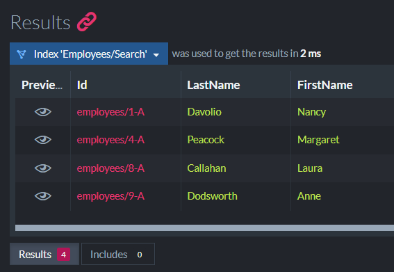
Which returns the following results:

image

Why did we get this particular employees?  Let’s find out:

image

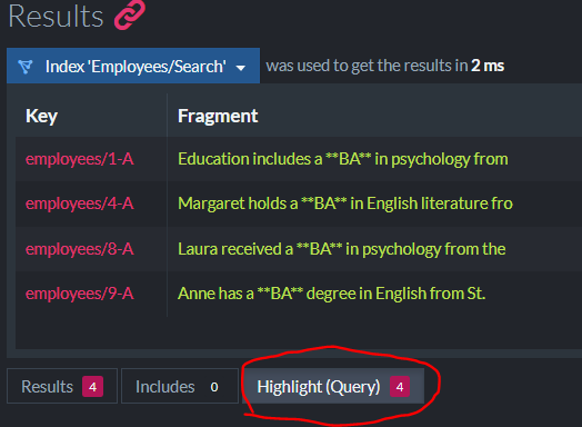
Now we are asking the server to highlight for us the reason for the match. You can see this in the studio directly, in the Highlight tab:

image

Using this approach, you can enrich the search result and provide nicer experience for your users.

time to read 1 min | 66 words

Just to let you know, the book is pretty much edited, that means that you won’t have to suffer through my horrible sentence structure.

You can read this here.

What remains to be done now is for me to go over the book again, verify that there aren’t any issues, and we are done.

In other words, we are now “Done, Done” in the “Done, Done, Done” scale.

time to read 3 min | 597 words

Rafal had a great comment on my previous post:

Much easier with humans in the process - just tell them to communicate and they will figure out how to do it. Otherwise they wouldn't be in the shoe selling business. Might be shocking for the tech folk, but just imagine how many pairs of shoes they would have to sell to pay for a decent IT system with all the features you consider necessary. Of course at some point the cost of not paying for that system will get higher than that…

This relates to have a chain of shoe stores that need to sync data and operations among the different stores.

Indeed, putting a human in the loop can in many cases be a great thing. A good example of that can be in order processing. If I can write just the happy path, I can be done very quickly. Anything not in the happy path? Let a human deal with that. That cut down costs by so much, and it allow you to make intelligent decisions on the spot, with full knowledge of the specific case. It is also quite efficient, since most orders fall into the happy path. It also means that I can come back in a few months and figure out what the most common reasons to fall off the happy path are and add them to the software, reducing the amount of work I shell to humans significantly.

I wish that more systems were built like that.

It is also quite easy to understand why they aren’t built with this approach. Humans are expensive. Let’s assume that we can pay a minimum wage, in the states, that would translate to about 20,000 USD. Note that I’m talking about the actual cost of employment, this calculation includes the salary, taxes, insurance, facilities, etc. If I need this to be a 24/7, I have to at least triple it (without accounting for vacation, sick leave, etc).

At the same time, x1e.16xlarge machine on AWS with 64 cores and 2 TB of memory will set me back by 40,000 a year. And it will likely be able to process transactions much faster than the two minimum wage employees that the same amount of money will get me.

Consider the case of a shoe store and misdirected check scenario, we need to ensure that the people actually receiving the check understand that this is meant for the wrong store and take some form of action. That means that we can just take Random Joe Teenager off the street. So another aspect to consider is the training costs. That usually means getting higher quality people and training them on your policies. All of which take quite a bit of time and effort. Especially if you want to have consistent behavior across the board.

Such a system, taken to extreme, result in rigid policy without a lot of place for independent action on the part of the people doing the work. I wish I could say that taking it to extreme was rare, but all you have to do is visit the nearest government office or bank or the post office to see common examples of people working working within very narrow set of parameters. The metric for that, by the way, is the number of times that you hear: “There is nothing I can do, these are the rules” per hour.

In such a system, it is much cheaper to have a rigid and inflexible system running on a computer. Even with the cost of actually building the system itself.

FUTURE POSTS

  1. Partial writes, IO_Uring and safety - about one day from now
  2. Configuration values & Escape hatches - 5 days from now
  3. What happens when a sparse file allocation fails? - 7 days from now
  4. NTFS has an emergency stash of disk space - 9 days from now
  5. Challenge: Giving file system developer ulcer - 12 days from now

And 4 more posts are pending...

There are posts all the way to Feb 17, 2025

RECENT SERIES

  1. Challenge (77):
    20 Jan 2025 - What does this code do?
  2. Answer (13):
    22 Jan 2025 - What does this code do?
  3. Production post-mortem (2):
    17 Jan 2025 - Inspecting ourselves to death
  4. Performance discovery (2):
    10 Jan 2025 - IOPS vs. IOPS
View all series

Syndication

Main feed Feed Stats
Comments feed   Comments Feed Stats
}